Components of time series#
A time series is a discrete time sequence of data points indexed in time which can be used to study a phenomenon. It is a record of the data collected at different points in time, it consists of discrete time samples of typically a continuous-time phenomenon in reality. The data are usually collected at fixed time intervals rather than just recording them intermittently or randomly. The fixed interval \(\Delta t\), in the time domain, is defined as ‘sampling interval’ and, in the frequency domain, is defined as ‘sampling rate’ or ‘sampling frequency’, expressed for example in Hz.
A time series is denoted as
The \(Y(t_i)\) are random variables, since the data is affected by noise.
The time instants, also defined as epochs, are \(t_i = i \Delta t\), indicating that the samples are equally spaced in time intervals of \(\Delta t\). Assuming a unit time interval (i.e., \(\Delta t=1\)), then \(t_i = i\) and we can write the time series as
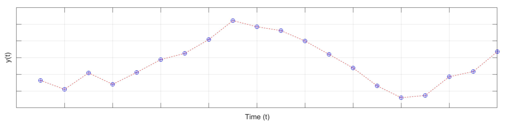
Fig. 2 Example of time series with equally spaced time interval \(\Delta t\)#
A time series can be decomposed as follows:
where we distinguish the following components:
\(tr(t)\) = trend, provides the general behavior and variation of the process
\(s(t)\) = seasonality, shows the regular seasonal variations
\(o(t)\) = offset, is a discontinuity (or jump) in the data
\(b(t)\) = irregularities and outliers (also referred to as biases), due to unexpected reasons. Irregularities will not be considered in this book.
\(\epsilon(t)\) = noise process, can be white or colored noise.
Trend#
The trend is the general pattern of the time series and shows its long-term changes. The trend can be linear, however higher order polynomials are also possible.
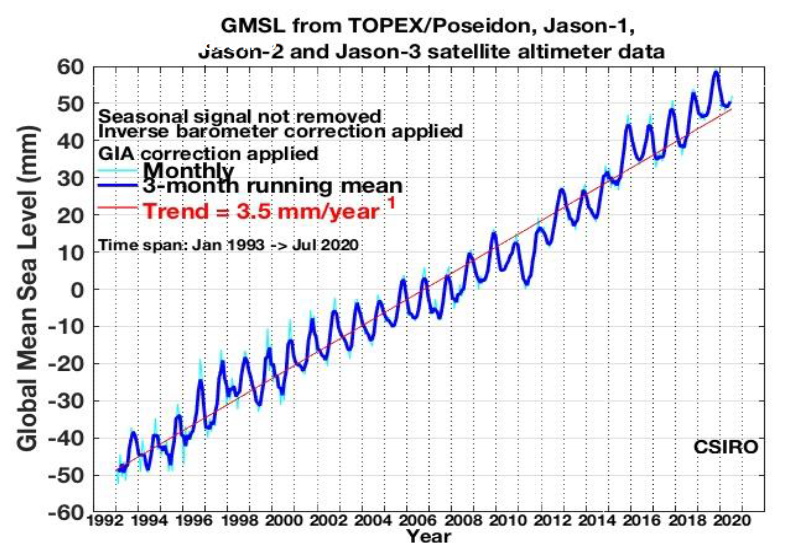
Fig. 3 Monthly time series of global mean sea level measurements using Satellite Altimetry technique. Source image: https://www.cmar.csiro.au/sealevel/sl_hist_last_decades.html#
Fig. 3 shows a positive trend (red line) of around \(3.5\) mm/year, which in this case indicates sea level rise. This however needs to be further investigated and tested statistically (see hypothesis_testing and also Modelling and Estimation).
Trend analysis expresses the changes of the variable of interest with respect to time \(t\). Different types of trend are possible and for now we will mainly focus on linear trend, i.e. the time-dependent variable \(Y(t)\) changes at a (constant) linear rate over time: \(Y_t = y_0 + r t + \epsilon_t\). Other trends are however also possible, for example, quadratic, which includes \(c t^2\), or log linear \(\log(Y_t) = y_0 + r t + \epsilon_t\).
Seasonality#
Seasonal variations explain regular fluctuations in a certain period of time (e.g. a year), usually caused by climate and weather conditions (e.g. temperature, rainfall), cycles of seasons, customs, traditional habits, weekends, or holidays. For example, the weekly signal is usually evident in the volume of people engaged in shopping (likely more people prefer going shopping in the weekends)
From Fig. 3 it is also possible to see the seasonal variations: in fact sea levels are higher in summer and lower in winter. The annual warming/cooling cycle is the main contributor to these seasonal variations.
Regular seasonal variations in a time series might be handled by using a sinusoidal model with one or more sinusoids with frequency that may be known or unknown depending on the context. In fig Fig. 3, cyclical behavior with a period of 1 year can be observed. A harmonic model for seasonal variation can be of the following two equivalent forms (using that \(\cos(u+v)= \cos u \cos v - \sin u \sin v\)):
With the coefficients \(a_k = A_k\cos\theta_k\) and \(b_k=-A_k\sin\theta_k\), and where \(\omega_0\) is the base (fundamental) frequency of the seasonal variation and is fixed or is determined by Spectral Analysis. To be more specific, we can use the psd to determine the unknown frequencies.
Once \(\omega_ 0\) is set, the coefficients \(a_k \) and \(b_k\) can be determined using the least-squares method, since the equation is linear in \(a_k\) and \(b_k\). From this the original sinusoids can be obtained using:
Note
This transformation is necessary to make the seasonal component phase-independent. Using regular estimation methods, we cannot linearly estimate the phase of the sinusoidal function. However by transforming the sinusoidal function into a linear combination of sine and cosine functions, we can estimate the phase of the seasonal component.
Show that the time series
with given \(\omega_0\), can be rewritten as
and derive the formulation of \(A\) and \(\theta\).
Hint: you might need to know trigonometric identity \(\cos(u+v)=\cos(u)\cos(v)-\sin(u)\sin(v)\)
Solution
Using the trigonometric identity to rewrite:
\( Y(t)=A \cos(\omega_0 t + \theta) = A (\cos(\omega_0 t)\cos(\theta)-\sin(\omega_0 t)\sin(\theta)) \)
Retrieving the functions for a and b
\( a = A \cos(\theta) \hspace{1cm} b = -A \sin(\theta)\)
Squaring both functions in order to get rid of the sin and cos
\( a^2 = A^2 \cos^2(\theta) \hspace{1cm} b^2 = A^2 \sin^2(\theta) \)
Adding both functions together
\( a^2 + b^2 = A^2 (\cos^2(\theta) + \sin^2(\theta)) \)
Using this property to simplify:
\( \cos^2(\theta) + \sin^2(\theta) = 1 \)
\( a^2 + b^2 = A^2 \)
Take square root to find A
\( \sqrt{a^2 + b^2} = A \)
For \(\theta\) we rewrite the second function
\( a = A \cos(\theta) \hspace{1cm} -b = A \sin(\theta)\)
\( \frac{-b}{a} = \frac{\sin(\theta)}{\cos(\theta)} = \tan(\theta) \)
\( \theta = \arctan(\frac{-b}{a}) \)
This video includes the solution to this exercise.
Offset (jump)#
Offsets are sudden changes or shifts in time series. There are different underlying reasons why we encounter offsets in time series.
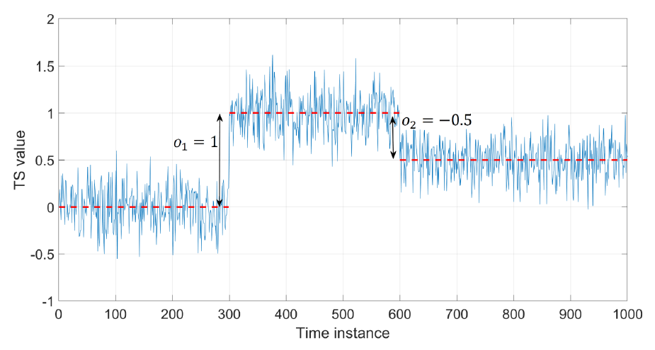
Fig. 4 Example of time series with two offsets.#
As a deterministic sudden change, offsets can be handled by a step function such as a heaviside step function with an epoch (time instant) that can be known or unknown (to be detected) depending on the time series.
In this case the time series is written as:
where \(q\) is the series of offsets (in Fig. 4 there are two offsets, hence \(q=2\)) and each of them is expressed as a Heaviside step function
Once the time instant (\(t_k\)) of the offset is known, the amplitude can be estimated using least-squares.
Noise#
Noise simply refers to random fluctuations in the time series about its typical pattern. In general we can talk about white and colored noise in time series analysis. The following characteristics are associated with noise:
Noise is not synonymous with error, although random variation, including measurement errors, contributes to noise. Essentially, noise represents the unpredictable fluctuations in data, while errors encompass any inaccuracies that may arise from a range of factors, including both random variations and systematic issues.
It is required to filter out unwanted random variations, and detect meaningful information (i.e., a signal) from noise processes.
Transforming data from the time domain to the frequency domain allows to filter out the frequencies that pollute the data.
White noise can be decomposed into its constituent components (frequencies). In principle, white noise contains all wavelengths/colors (like white light), each contributing equally to the fluctuations observed in the data.
Colored noise can seriously affect the analysis of time series, and their parameters of interest. Short-term colored noise has also predictive property (used for forecasting).
A purely stationary random process (or white noise process) yields a sequence of uncorrelated zero-mean random variables. This zero-mean random process is of the form
where \(\epsilon_t\) is the independent identically distributed (i.i.d.) error at epoch \(t\). Therefore, the observation/noise at time \(t\) is not dependent on any of the previous observations \(Y_t\).
Stochastic model#
A stationary zero-mean random process has an expectation of zero (functional model), and a scaled identity matrix as its covariance matrix (stochastic model). The functional and stochastic models of white noise are of the form
and
The noise can be represented with, for example, a Gaussian distribution with mean \(\mu=0\) and variance \(\sigma^2\), that is \(\epsilon(t) \sim \textbf{N}(0, \sigma^2)\).
It can be written as
where
\(y_0\) is the intercept (e.g. in mm)
\(r\) is the rate (e.g. in mm/year)
\(a\) and \(b\) are the coefficients of the signal, (e.g. annual signal)
\(\omega_0\) is the frequency (e.g. 1 cycle/year)
\(o\) is the offset starting at time \(t_k\)
\(u_k(t)\) is the Heaviside step function
\(\epsilon(t)\) is the i.i.d. random Gaussian noise, i.e. \(\epsilon(t) \sim \textbf{N}(0, \sigma^2)\).