Time Series Stationarity

Definition

A stationary time series is a stochastic process whose statistical properties do not depend on the time at which it is observed.

This means that parameters such as mean and (co)variance should remain constant over time and not follow any trend, seasonality or irregularity.

• Mean of the process is time-independent

\[\mathbb{E}(S(t))=\mathbb{E}(S_t)=\mu\]

• Covariance of the process is independent of \(t\) for each time shift \(\tau\) (so only a function of τ and not t):

\[ Cov(S_t,S_{t-\tau})= Cov(S_t,S_{t+\tau}) =\mathbb{E}((S_t-\mu)(S_{t-\tau}-\mu))=c_\tau \]

• The variance (i.e., \(\tau=0\)) is then also constant with respect to time :

\[ Var(S_t)=\mathbb{E}((S_t-\mu)^2)=c_0=\sigma^2 \]

Notice that we have introduced the new notation \(S_t\) to denote a stationary time series. The time series \(Y_t\) is then a non-stationary time series.

Why stationary time series?

Stationarity is important if we want to use a time series for forecasting (predicting future behaviour), which is not possible if the statistical properties change over time.

In practice, we may in fact be interested in for instance the trend and seasonality of a time series. Also, many real-world time series are of course non-stationary. Therefore the approach is to first “stationarize” the time series (e.g., remove the trend), use this stationary time series to predict future states based on the statistical properties (stochastic process), and then apply a back-transformation to account for the non-stationarity (e.g., add back the trend).

How to “stationarize” a time series?

There are several ways to make a time series stationary. In this course we will focus on detrending the data using least-squares fit.

Least-squares fit

If we can express the time series \(Y=[Y_1, ..., Y_m]^T\) with a linear model of observation equations as \(Y = \mathrm{Ax} + \epsilon\), we can apply best linear unbiased estimation to estimate the parameters \(\mathrm{x}\) that describe e.g. the trend and seasonality:

\[ \hat{X}=(\mathrm{A}^T\Sigma_{Y}^{-1}\mathrm{A})^{-1}\mathrm{A}^T\Sigma_{Y}^{-1}Y \]

A detrended time series is obtained in the form of the residuals

\[ \hat{\epsilon} = Y - \mathrm{A}\hat{X} \]

The detrended \(\hat{\epsilon}\) is assumed to be stationary for further stochastic processing. This is also an admissible transformation because \(Y\) can uniquely be reconstructed as \(Y=\mathrm{A}\hat{X}+\hat{\epsilon}\).

Let us take a look into an example:

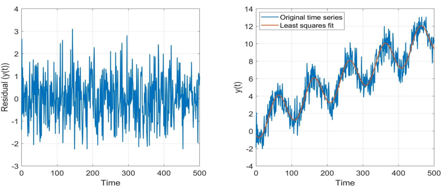
Fig. 7 Example of a time series (right graph) with linear and seasonal trend. The residuals (= stationary time series) after applying BLUE are shown on the left.

In the example above, for each observation \(Y_i = y_0+ rt_i+a\cos{\omega_0t_i}+b \sin{\omega_0t_i} +\epsilon_i\), where \(a\) and \(b\) describe the seasonality and \(y_0\) and \(r\) the trend. The time series then is:

\[\begin{split} \begin{bmatrix} Y_1 \\ Y_2 \\ \vdots \\ Y_m \end{bmatrix} = \begin{bmatrix} 1&t_1&\cos{\omega_0 t_1} & \sin{\omega_0 t_1} \\ 1&t_2&\cos{\omega_0 t_2} & \sin{\omega_0 t_2} \\ \vdots & \vdots & \vdots & \vdots \\ 1&t_m&\cos{\omega_0 t_m} & \sin{\omega_0 t_m} \end{bmatrix} \begin{bmatrix} y_0 \\ r \\ a \\ b \end{bmatrix} + \begin{bmatrix} \epsilon_1 \\ \epsilon_2 \\ \vdots \\ \epsilon_m \end{bmatrix} \end{split}\]

The time series of residuals (left panel) is indeed a stationary time series.

Other ways to make a time series stationary

When model specification is not straightforward, other methods can be used to make a time series stationary. Two common methods are single differencing and moving average. Single differencing of \(Y=[Y_1,...,Y_m]^T\) makes a time series \(\Delta Y_t=Y_t - Y_{t-1}\). Another way to create an (almost) stationary time series is by taking the moving average of the time series. Where we apply a moving average of \(k\) observations to the time series \(Y\) to create a new time series \(\bar{Y}_t = \frac{1}{k}\sum_{i=1}^{k}Y_{t-i}\), and then take the difference between the original time series and the moving average to obtain a (nearly) stationary time series \(\Delta Y_t = Y_t - \bar{Y}_t\).

Both these methods do not require a model specification. So in cases where the model is not known, these methods can be used to make the time series stationary.

… and then what?

We have seen different ways of obtaining a stationary time series from the original time series. The reason is that in order to make predictions (forecasting future values, beyond the time of the last observation in the time series) we need to account for both the signal-of-interest and the noise. Estimating the signal-of-interest was covered in the previous section. In the next sections we will show how the noise can be modelled as a stochastic process. Given a time series \(Y=\mathrm{Ax}+\epsilon\), the workflow is as follows:

1. Estimate the signal-of-interest \(\hat{X}=(\mathrm{A}^T\Sigma_{Y}^{-1}\mathrm{A})^{-1}\mathrm{A}^T\Sigma_{Y}^{-1}Y\) (Section Modelling and estimation).

2. Model the noise using the Autoregressive (AR) model, using the stationary time series \(S:=\hat{\epsilon}=Y-\mathrm{A}\hat{X}\) (Section AR).

3. Predict the signal-of-interest: \(\hat{Y}_{signal}=\mathrm{A}_p\hat{X}\), where \(\mathrm{A}_p\) is the design matrix describing the functional relationship between the future values \(Y_p\) and \(\mathrm{x}\) (Section Forecasting).

4. Predict the noise \(\hat{\epsilon}_p\) based on the AR model.

5. Predict future values of the time series: \(\hat{Y}_p=\mathrm{A}_p\hat{X}+\hat{\epsilon}_p\) (Section Forecasting).