Modelling and Estimation

The goal is now to:

• estimate parameters of interest (i.e., components of time series) using Best Linear Unbiased Estimation (BLUE);

• evaluate the confidence intervals of the estimators for the parameters of interest;

Components of time series

As already discussed, we will distinguish the following components in a time series:

• Trend: General behavior and variation of the process. This often is a linear trend with an unknown intercept \(y_0\) and a rate \(r\).

• Seasonality: Regular seasonal variations, which can be expressed as sine functions with (un)known frequency \(\omega\), and unknown amplitude \(A\) and phase \(\theta\), or with unknowns \(a(=A\sin\theta)\) and \(b(=A\cos\theta)\).

• Offset: A jump of size \(o\) in a time series starting at epoch \(t_k\).

• Noise: White or colored noise (e.g., AR process).

Best Linear Unbiased Estimation (BLUE)

#TODO: add reference to the chapter on estimation

If the components of time series are known, we may use the linear model of observation equations to estimate those components.

Consider the linear model of observation equations as

\[Y=\mathrm{Ax}+\epsilon, \hspace{10px} \mathbb{D}(Y)=\Sigma_{Y}\]

Recall that the BLUE of \(\mathrm{x}\) is:

\[\hat{X}=(\mathrm{A}^T\Sigma_{Y}^{-1}\mathrm{A})^{-1}\mathrm{A}^T\Sigma_{Y}^{-1}Y,\hspace{10px}\Sigma_{\hat{X}}=(\mathrm{A}^T\Sigma_{Y}^{-1}\mathrm{A})^{-1}\]

The BLUE of \(Y\) and \(\epsilon\) is

\[\hat{Y}=\mathrm{A}\hat{X},\hspace{10px}\Sigma_{\hat{Y}}=\mathrm{A}\Sigma_{\hat{X}}\mathrm{A}^T\]

and

\[\hat{\epsilon}=Y-\hat{Y},\hspace{10px}\Sigma_{\hat{\epsilon}}=\Sigma_{Y}-\Sigma_{\hat{Y}}\]

Model of observation equations

The linear model, consisting of the above three components plus noise, is of the form

\[Y_t = y_0+rt+a\cos{\omega t}+b\sin{\omega t}+ou_k(t)+\epsilon_t\]

The linear model should indeed be written for all time instances \(t_1,...,t_m\), resulting in \(m\) equations as:

\[\begin{split} \begin{align*} Y(t_1) &= y_0+rt_1+a\cos{\omega t_1}+b\sin{\omega t_1}+ou_k(t_1)+\epsilon(t_1)\\ Y(t_2) &= y_0+rt_2+a\cos{\omega t_2}+b\sin{\omega t_2}+ou_k(t_2)+\epsilon(t_2)\\ &\vdots \\ Y(t_k) &= y_0+rt_k+a\cos{\omega t_k}+b\sin{\omega t_k}+ou_k(t_k)+\epsilon(t_k)\\ &\vdots \\ Y(t_m) &= y_0+rt_m+a\cos{\omega t_m}+b\sin{\omega t_m}+ou_k(t_m)+\epsilon(t_m) \end{align*} \end{split}\]

These equations can be written in a compact matrix notation as

\[Y=\mathrm{Ax}+\epsilon\]

where

\[\begin{split} \overbrace{\begin{bmatrix} Y_1\\ \vdots\\ Y_{k-1}\\ Y_k\\ \vdots\\ Y_m\end{bmatrix}}^{Y} = \overbrace{\begin{bmatrix} 1&t_1&\cos{\omega t_1}&\sin{\omega t_1}&0 \\ \vdots&\vdots&\vdots&\vdots&\vdots\\ 1&t_{k-1}&\cos{\omega t_{k-1}}&\sin{\omega t_{k-1}}&0\\ 1&t_k&\cos{\omega t_k}&\sin{\omega t_k}&1\\ \vdots&\vdots&\vdots&\vdots&\vdots\\ 1&t_m&\cos{\omega t_m}&\sin{\omega t_m}&1\end{bmatrix}}^{\mathrm{A}}\overbrace{\begin{bmatrix}y_0\\ r\\ a\\ b\\ o\end{bmatrix}}^{\mathrm{x}}+\overbrace{\begin{bmatrix}\epsilon_1\\ \vdots\\ \epsilon_{k-1} \\ \epsilon_k\\ \vdots\\ \epsilon_m\end{bmatrix}}^{\epsilon}\end{split}\]

with the \(m\times m\) covariance matrix

\[\begin{split}\Sigma_{Y}=\begin{bmatrix}\sigma_1^2&\sigma_{12}&\dots&\sigma_{1m}\\ \sigma_{21}&\sigma_{2}^2&&\\ \vdots&\vdots&\ddots&\\ \sigma_{m1}&\sigma_{m2}&\dots&\sigma_{m}^2\end{bmatrix}\end{split}\]

Exercise

A time series exhibits a linear regression model \(Y(t)=y_0 + rt + \epsilon(t)\). The measurements have also been taken at a measurement frequency of 10 Hz, producing epochs of \(t=0.1,0.2, \dots,100\) seconds, so \(m=1000\). Later an offset was also detected at epoch 260 using statistical hypothesis testing. For the linear model \(Y=\mathrm{Ax}+\epsilon\), establish an appropriate design matrix that can capture all the above effects.

Solution

In the linear regression case, the design matrix consists of two columns, one for the unknown \(y_0\) (a column on ones), and the other for \(r\) (a column of time, \(t\)). Due to the presence of an offset, the mathematical model should be modified to:

\[ Y(t) = y_0 +rt +o_k u_k(t) + \epsilon(t) \]

where \(u_k(t)\) is the Heaviside step function:

\[\begin{split} u_k(t) = \begin{cases} 0, & \textrm{if} & t<t_k=26 \\ 1, & \textrm{if} & t\geq t_k=26 \end{cases} \end{split}\]

and \(o_k\) is the magnitude of the offset. This means that we have to add a third column to the design matrix having zeros before the epoch 260, and ones afterwards. Since epoch 260 corresponds to \(t=26\) s (noting that we have 10 Hz data), in \(\mathrm{A}\) we begin to have 1’s in that row:

\[\begin{split} \mathrm{A} = \begin{bmatrix} 1 & t_1 & 0 \\ \vdots & \vdots & \vdots\\ 1 & t_{259} & 1\\ 1 & t_{260} & 1\\ \vdots & \vdots & \vdots \\ 1 & t_{1000} & 1 \\ \end{bmatrix} = \begin{bmatrix} 1 & 0.1 & 0 \\ \vdots & \vdots & \vdots\\ 1 & 25.9 & 0 \\ 1 & 26 & 1\\ \vdots & \vdots & \vdots \\ 1 & 100 & 1 \\ \end{bmatrix} \end{split}\]

Estimation of parameters

If we assume the covariance matrix, \(\Sigma_{Y}\), is known, we can estimate \(\mathrm{x}\) using BLUE:

\[\begin{split}\hat{X}=\begin{bmatrix}\hat{y_0}\\ \hat{r}\\ \hat{a}\\ \hat{b}\\ \hat{o}\end{bmatrix},\hspace{10px}\Sigma_{\hat{X}}=\begin{bmatrix}\sigma_{\hat{y}_0}^2& \sigma_{\hat{y}_0\hat{r}}& \sigma_{\hat{y}_0\hat{a}}& \sigma_{\hat{y}_0\hat{b}}& \sigma_{\hat{y_0}\hat{o}}\\ \sigma_{\hat{r}\hat{y}_0}& \sigma_{\hat{r}}^2& \sigma_{\hat{r}\hat{a}}& \sigma_{\hat{r}\hat{b}}& \sigma_{\hat{r}\hat{o}}\\ \sigma_{\hat{a}\hat{y_0}}& \sigma_{\hat{a}\hat{r}}& \sigma_{\hat{a}}^2& \sigma_{\hat{a}\hat{b}}& \sigma_{\hat{a}\hat{o}}\\ \sigma_{\hat{b}\hat{y_0}}& \sigma_{\hat{b}\hat{r}}& \sigma_{\hat{b}\hat{a}}& \sigma_{\hat{b}}^2& \sigma_{\hat{b}\hat{o}}\\ \sigma_{\hat{o}\hat{y_0}}& \sigma_{\hat{o}\hat{r}}& \sigma_{\hat{o}\hat{a}}& \sigma_{\hat{o}\hat{b}}& \sigma_{\hat{o}}^2\end{bmatrix}\end{split}\]

Given \(\hat{X}\) and \(\Sigma_{\hat{X}}\), we can obtain the confidence region for the parameters. For example, assuming the observations are normally distributed, a 99% confidence interval for the rate \(r\) is (\(\alpha=0.01\)):

\[\hat{r}\pm k\sigma_{\hat{r}}\]

where \(\sigma_{\hat{r}} = \sqrt{(\Sigma_{\hat{X}})_{22}}\) is the standard deviation of \(\hat{r}\) and \(k=2.58\) is the critical value obtained from the standard normal distribution (using \(0.5\alpha\)).

Model identification

The design matrix \(\mathrm{A}\) is usually assumed to be known. So far, we have assumed the frequency \(\omega\) of the periodic pattern (seasonality, for example) in a \(a\cos{\omega t} + b\sin{\omega t}\) is known, so the design matrix \(\mathrm{A}\) can be directly obtained. In some applications, however, such information is hidden in the data, and needs to be identified/detected. Linear model identification is a way to reach this goal.

How to determine \(\omega\) if it is unknown a priori?

Example power spectral density

Fig. 6 shows on the left the original time series as well as the estimated linear trend and seasonal signal. The sine wave has a period (\(T=1/f\)) of 100. Indeed the PSD as function of period on the right shows a peak at a period of 100.

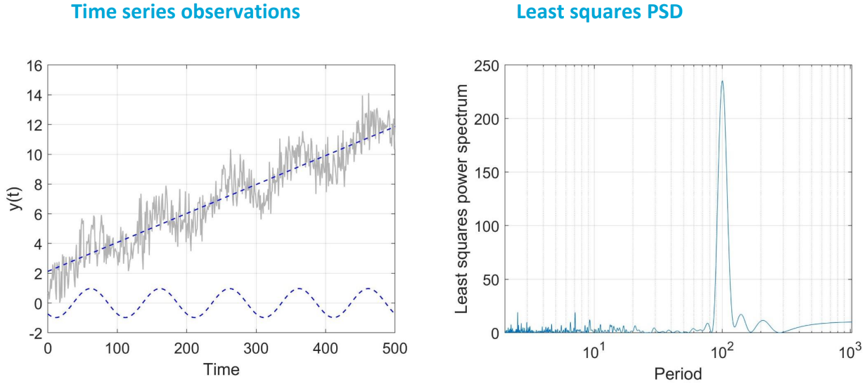
Fig. 6 Left: time series (grey) and estimated linear trend and sine wave with period of 100. Right: estimated PSD.

This means we can estimate the frequency \(\omega\) of the periodic pattern using the techniques discussed in the chapter on signal processing. Once we have the frequency, we can construct the design matrix \(\mathrm{A}\).

It is also possible to infer the frequency of the periodic pattern by reasoning. For example, if we know our model depends on temperature, we can assume that the frequency of the seasonal pattern is related to the temperature cycle (e.g., 24 hours). However, this is a more qualitative approach and should be used with caution. Best practice is to use the DFT or PSD to estimate the frequency.